In a previous post I explained how to install RStudio, a popular integrated development environment for the R programming language.
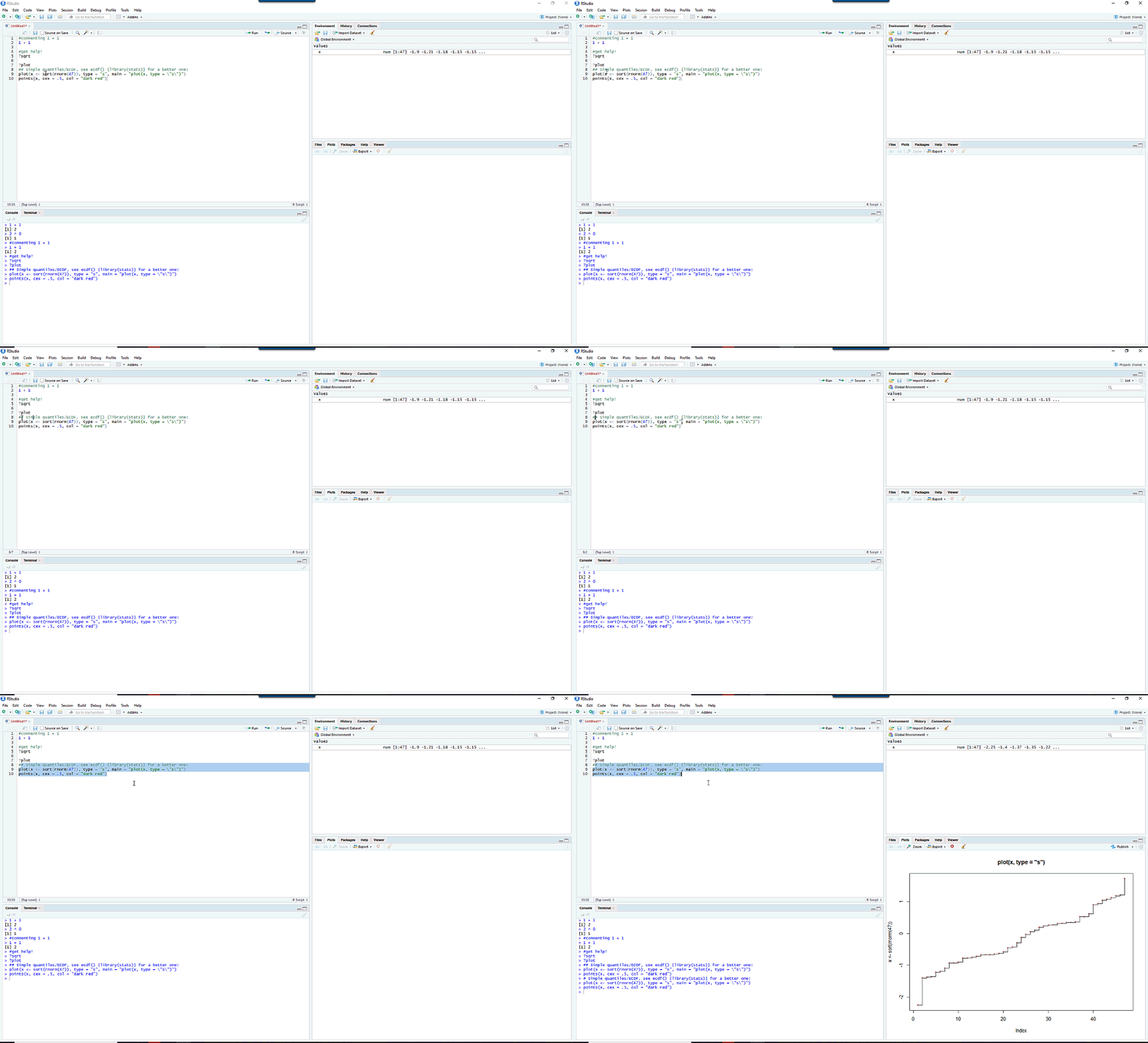
Open up RStudio for the first time and it might look like some mad scientist’s Mission Control. In this post I will walk through each pane and what it does. From this you will start to see just what is so “integrated” about this integrated development environment.
0. The blank slate

When you open up RStudio for the first time you should see something like the above. If you do not see a window on the upper-left hand side, open a new script with the keyboard shortcut Ctrl + Shift + N on Windows.
What do all these panes mean? We will cover what each of them do.
1. The console
In the lower left-hand corner of RStudio. This is where commands are submitted to R to execute.
Here you will see the “>” sign followed by a blinking cursor. Enter your operations here and then press “Enter” to send them to the console.
In my free-mini course I dig a bit deeper into operating in the R console.
2. The script editor
While you can operate directly from the console, it’s often a good idea to write them in a script and then send them to the console. This way you can save a long-term record of the code you ran.
a. Commenting code
Another nice feature here is to leave comments in your script by starting the line with the “#” character. These lines will not be executed and are instead notes for the programmer.
b. Running code
Place your cursor anywhere in the line of the code you want to send to the console to execute.
To run this code, click the Run button at the top of the script editor. You can also use Ctrl + Enter in RStudio.
I prefer the older shortcut Ctrl + R to run code. To change your keyboard shortcut setting you can go to Tools | Modify Keyboard Shortcuts. Find the selection for “Run Current Line or Selection” and change the shortcut by keying “Ctrl + R” in instead of “Ctrl + Enter.”
You can also run multiple lines of code at the same time by highlighting and running all of them.
Finally, save your R script by going to File | Save or with the Ctrl + S keyboard shortcut.
3. The files/packages/plot pane
Next we move to the lower right-hand side of RStudio.
a. Getting help
The help tab in this pane is particularly useful. It returns a help file when you use a “?” in front of a function in your command prompt. (You can also use the the help() function to get more information about a given function.)
In this example we will search for the sqrt function. In the help pane we now see R’s documentation on this function.
Suggested post: “5 Ways to Get Help in R”
b. Plots
This tab will hold any plots you create in your R section. For now we will use the ? command to get help on the plot function itself.
Scrolling down the help documentation on the plot function, you will see a few examples. Let’s run the final example:
#last example from R's help documentation on the plot function:

## Simple quantiles/ECDF, see ecdf() {library(stats)} for a better one:
plot(x <- sort(rnorm(47)), type = "s", main = "plot(x, type = \"s\")")
points(x, cex = .5, col = "dark red")
Running this code you will now see a plot in the Plot tab of the lower right hand pane. With the buttons above you can do things like export the plot or zoom in on it.
4. The environment
Last but not least, let’s check out the Environment tab on the upper right hand side of RStudio.
a. The History tab
Here you will see a history of all the commands you have sent to the R console in your session.
You can send a line back to your editor script or to the console. You can also save the entire R history page as a special R History file.
b. The environment tab
This is a list of all loaded R objects.
Right now you will see R has an object called “x.” Where did this object come from? You created this when you copied and ran code from the plot function example.
Objects are largely what make R, R. Everything in R is stored as an object and to access values you must first assign them as objects.
Suggested reading: Creating objects and assigning values in R
Let’s go ahead and create one more object: one called “result” that holds the square root of 25.
You will see that the new object is added to our Environment tab.
You can clear all objects in your environment with the broom at the top of the Environment tab. If you wanted to clear just one object, use the rm(x) function in your R script.
Bonus! RStudio Settings
Under Tools | Global Options you have the choice to change some program settings. While you are not likely to change most of these here are a couple to note:
- Pane Layout: Here you can adjust the layout of panes and windows in RStudio. I like how they are by default, but it is worth experimenting with.
- Appearance: This one is fun to play around with. Here you can change the theme and appearance of your RStudio environment. Check out the many editor themes to break out of the normal black-on-white environment. (I am partial to the Merbivore theme editor — not only do I like that the black background cuts down on glare, I like the Halloween-y fonts used.)
Getting integRated
With this post I hope you are starting to see how the various panes and windows in RStudio connect. For more on R, check out my free mini-course or browse my previous posts on R.


