Table time! Reasons to start using Excel tables now

One of the first practices I encourage Excel users to pick up is to store all their data in tables.

Tables can take some getting used to, especially for those used to the traditional relative and absolute references (A1:B2, $B$4:$C$10, etc). But the adoption is totally worth it — both for what they can do in Excel, and what they prepare you for next.

In this introductory demo to Excel tables, you’ll be working with real world wholesale customers data from the UC Irvine Machine Learning repository.

They remind you to include headers

Receiving a dataset without any column headers is pretty useless, right? How are you supposed to make any sense of the data when the data isn’t measured?

Yet I’m sure you’ve received a dataset breaking this very cardinal rule.

Excel tables serve as a great reminder that a table is only as good as its headers.

Take a look at the start worksheet of the demo workbook — we have a series of data in columns A:F but with no headers — those are tucked away in columns H:L for now. Not a great look.

Go ahead and click anywhere in the main data source, then head to Insert > Tables > OK. The keyboard shortcut is Ctrl + T.

You may notice that, automatically, the Create Table menu asks if your data has headers. If it doesn’t a header column is automatically added to the table:

From here, you can go ahead and copy-paste the headers from columns H:M into the main table. It’s now clear what’s being measured in each column.

Headers and footers are separate elements of the table

Are these header columns part of the dataset proper? To quote a famous meme… “yes, but actually no.” They’re more like metadata that tells us what the data is, rather than the data itself. Classic Excel formulas have no way to programatically distinguish data from headers… but Excel tables do.

Let’s try it out. Head over to cell H3 in your worksheet and hit the equals sign =. Drag cells A1:F1 as your reference, and you’ll see that the formula becomes Table1[#Headers].

Once you’ve established this reference to the headers of Table 1, you can even use “downstream” as a reference to other functions, such as UPPER() to dynamically convert the case of all headers.

Viewing the table footers

If every story contains a beginning, middle and end, then every Excel table consists of headers, data and footers… but footers need to be checked on manually.

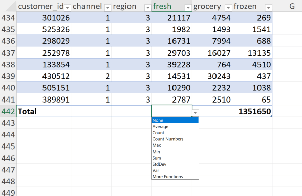
To do this, click anywhere in the table and go to Table Design on the ribbon, then check on Total Row in the Table Style Options group:

By default, this row will take a sum of the last column in your data, but you can click the dropdown menu on any of the columns to change:

Now that you have assembled the three elements of the table, confirm that you can “reconstruct” it using the following formulas:

As you advance your table skills, you’ll find still other useful formula references. But they all rely on the simple structure of headers, body and footers.

It forces you to use named ranges

It’s great to be able to programatically refer to the elements of a table… but not so great that this table has an uninspired name!

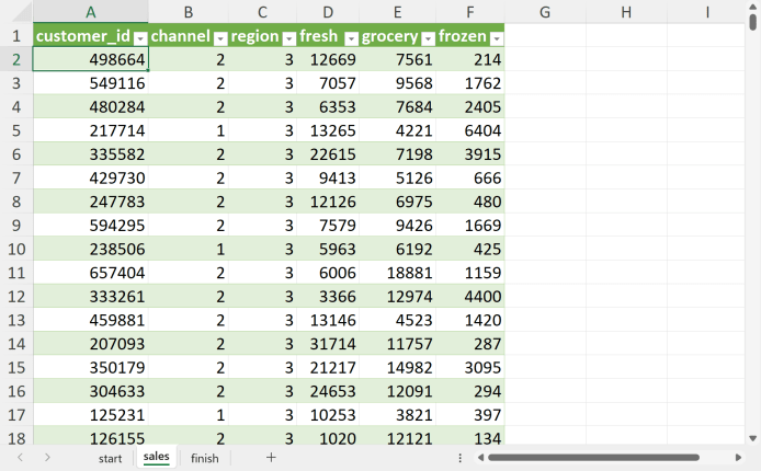
To be fair, it’s still better to refer to Table1 than cells A1:F22, for example. But if you’re going to name a range anything, it should be descriptive about the underlying data! Let’s go ahead and do this by heading to Formulas on the home ribbon, then Name Manager > Edit. Change the name to sales, then click OK. Click out of the Name Manager and you’ll see that every reference to Table1 has been changed to sales.

Excel tables must be named something. And while you can use the defaults, it’s a big win with little effort to provide a more meaningful name.

They look good

As an Excel user, your numbers are often only as good as their formatting. Using tables will instantly improve the aesthetics of your data by adding banded rows. Quickly and easily change the look and feel of the table by heading to Table Design in the ribbon:

This sure beats the tedious and error-prone process of trying to make the data look good on your own.

And, unlike a Maybelline makeover, Excel tables will stay put and looking good at the end of even the longest day…

You can easily add or remove data from the table

We’ve all been there before: you’ve got a total of some range in your workbook, that range changes because data is added to or deleted, that total breaks.

No more with Excel tables!

Here I have taken the sum of the fresh field using Excel tables’ structured references. I can add and remove data from sales and this formula maintains its integrity. Moreover, so does the total at the bottom, and it’s easy to exclude that total from my outside structured reference in cell I443.

Because we are referring to the data by object name, rather than location, it’s much less likely that manipulating the placement and dimensions of our table is going to adversely impact downstream formulas.

It’s the portal into Power Query

Does this sound like a familiar workflow? Every week you get a data extract that you need to report on. But first you’ve got to filter out rows, merge data sources, calculate columns… if so, you need to be using Power Query!

And guess what? The first step to do that is… to use tables.

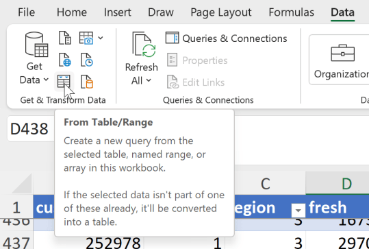
Click anywhere in the sales dataset, then go to Data > Get Data > From Table/Range. If this data weren’t already in a table, you’d have to do it now anyway!

You should now see a new screen called the Power Query Editor. This is a workhorse of a tool for data cleaning and preparation. For a more detailed tour of Power Query and the interface, check out this post.

One annoying thing about Power Query is that it imports the Totals row from the underlying Excel table, which can cause errors and easily double-count your data. To prevent this, go to Home on the ribbon, then Remove Rows > Remove Bottom Rows > 1:

Take a look at the Applied Steps menu to the right of your data and you’ll see “Removed Bottom Rows” has been added. Every action taken on the data can be traced and repeated from this menu, making Power Query a boon for automation. And it all started by converting your input data to a table!

One last thing to save your query — head to the Home tab of the ribbon, then click Close & Load. A new, “Power Queried” version of your data will get loaded to another worksheet as… a table!

This table has all of the same magical properties as the one you’ve seen before. That said, I wouldn’t make many changes to this one as any updating of your Power Query steps could wipe them out on refresh.

Tables really are the gateway to the automation dream factory that is Power Query.

Don’t table learning more tables

Were you able to follow along with all the cool stuff in this demo? Check your work below:

And while you’re at it, keep exploring tables! Try converting some of your existing workbooks to tables. Check out Microsoft’s documentation on the subject. And take those first steps into Power Query.

If you’re just getting started with tables, what questions do you have? Do you see any drawbacks from this approach to classic cell references? If tables have already won you over, what benefits did I miss? Please do let me know in the comments.