
When it comes to predictive modeling, Excel can take you surprisingly far. You can even build models like logistic regression natively. But when it comes to evaluating and validating those models, things get a lot trickier. Accuracy alone doesn’t tell the whole story, and digging into deeper metrics like precision, recall, F1-scores, or using cross-validation is either cumbersome or downright impossible to do with Excel’s built-in tools.
That’s where Copilot and Python in Excel come in. By combining Excel’s accessibility with Python’s statistical power, we can easily run the kinds of evaluation and validation steps that data professionals rely on to trust their models. In this post, we’ll look at a handful of these techniques such confusion matrices, cross-validation, precision and recall, and even comparing models like logistic regression and random forests.
To keep things concrete, we’ll use the Wisconsin Breast Cancer dataset, a classic dataset for classification problems. You can follow along using the exercise file linked below.
Recoding and checking the balance of the target variable
Our first task is to take the diagnosis column, which contains B for Benign and M for Malignant, and recode it into a numeric column we’ll call target. Here, 0 represents Benign and 1 represents Malignant. Here’s our prompt:
“In my dataset the diagnosis column has the values B for Benign and M for Malignant. Please create a new column called target that recodes these values into numbers, with 0 = Benign and 1 = Malignant. Then, count how many rows are in each group (0 vs 1) and tell me if the dataset looks balanced or if one class is much larger than the other.“
Why start here? Because before building any predictive model, it is critical to understand the shape of the data, especially how balanced the classes are. If one class, say Benign, appears much more often than the other, a model might simply learn to always guess Benign and still achieve deceptively high accuracy. By recoding the labels into numbers and counting how many cases fall into each group, we set ourselves up for meaningful evaluation later.

In this dataset there are 357 benign cases and 212 malignant ones. That means benign cases are somewhat more frequent, but malignant cases still make up a large share of the data. The split is not perfectly even, yet it is not so lopsided that the model will have trouble learning patterns for both outcomes.
What this tells us is that we can move forward with building models, but when it comes time to evaluate them we will want to use more than just accuracy, since the imbalance could cause accuracy alone to be misleading.
Train/test split
The next step is to split the dataset into two parts, one for training and one for testing. The idea is that the training set is used to fit the model, while the test set is held back until the very end. That way we can see how well the model performs on data it has never seen before, which is a much better check of whether it will generalize to new cases. We’ll prompt Copilot:
“Split the data into a training set (80%) and a test set (20%) so we can check our results on new data.”

In this case the dataset was divided using an 80/20 split, giving us 455 rows for training and 114 rows for testing. That means the model will have plenty of data to learn from while still leaving a meaningful chunk set aside for evaluation. This is a healthy balance that ensures we are not overfitting to the training data and gives us a fair way to measure the model’s accuracy on unseen examples.
Training a logistic regression model
With the data split into training and test sets, the next step is to actually fit a model. Logistic regression is a natural starting point for binary classification problems like this one, where the goal is to predict whether a diagnosis is benign or malignant.
After training the logistic regression model on the 455 training rows, we can check how it performs both on the training data and on the 114 rows in the test set. Looking at both is important. Accuracy on the training set shows how well the model fits the data it has already seen, while accuracy on the test set shows how well it generalizes to new, unseen cases.
“Train a logistic regression model using the training set to predict whether a diagnosis is Benign (0) or Malignant (1). Then, print the accuracy of the model on both the training set and the test set so we can see how well it performs on familiar data and on new data.”
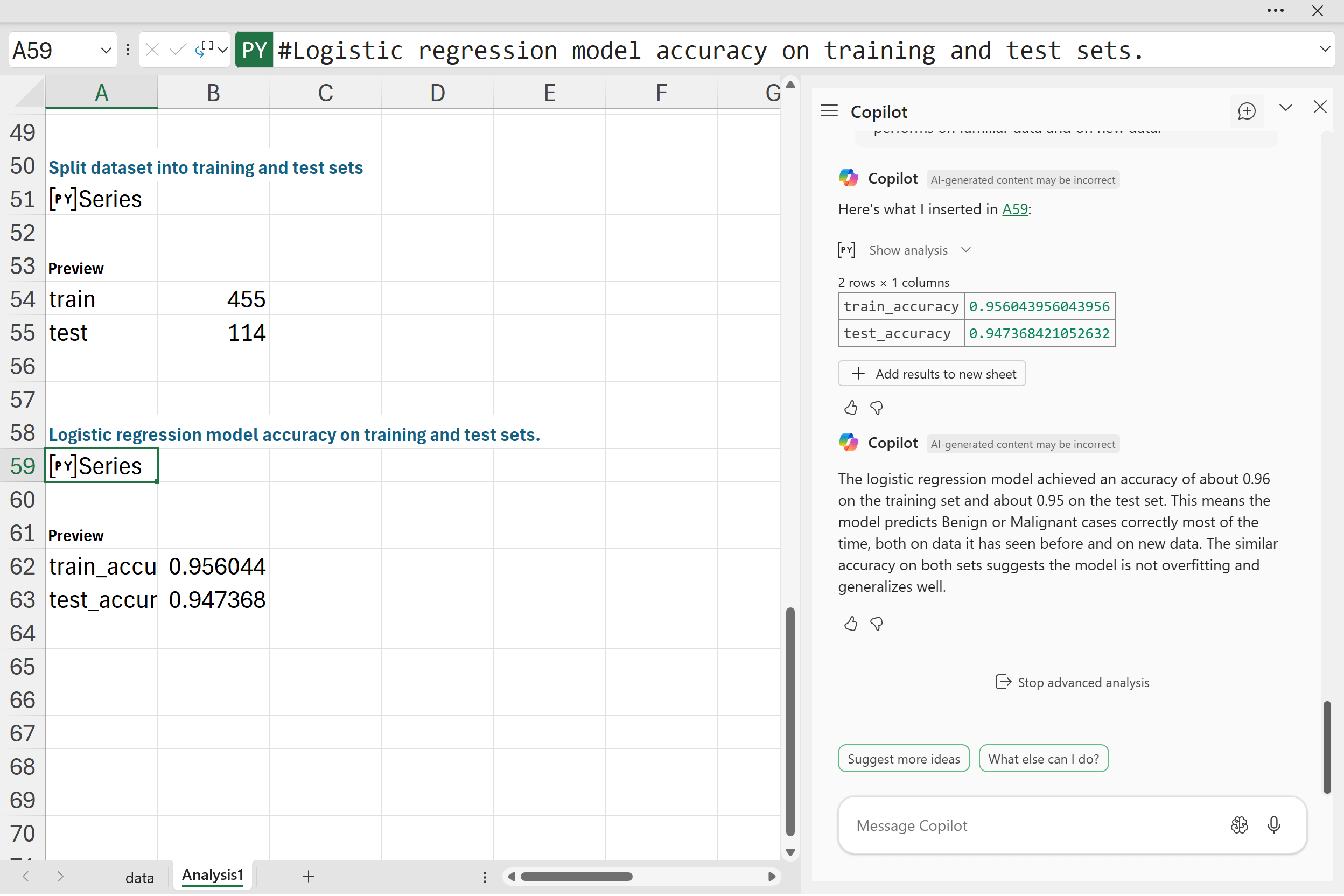
The results here show that the model achieved high accuracy on both the training and test sets. That means the logistic regression is capturing real patterns in the data rather than just memorizing the training cases. This balance is encouraging because it suggests the model will likely perform well on future diagnoses, not just the data we gave it to learn from.
K-fold validation
Up to this point we have looked at one train/test split, which gave us a good first check of how well the model generalizes. But a single split can sometimes give an incomplete picture. If the test set happens to be unusually easy or difficult, the accuracy might look better or worse than it really is.
To get a more reliable estimate of model performance, we can use cross-validation. In 5-fold cross-validation the data is divided into five parts. The model is trained on four of them and tested on the remaining one, and this process is repeated five times so that every part of the data gets used as a test set once. The final accuracy is then averaged across all five runs.
“Instead of just one train/test split, use 5-fold cross-validation with logistic regression. Print the average accuracy across all 5 runs.”

Here the logistic regression model achieved an average accuracy of about 95 percent across the five folds. This confirms that the earlier results were not just a fluke of the particular train/test split. It shows that the model is consistently able to classify new cases with high accuracy no matter how the data is divided, which gives us more confidence in its reliability.
Confusion matrix
So far we have looked at overall accuracy, but that only tells part of the story. A confusion matrix breaks the results down into exactly how many cases were predicted correctly and where the model made mistakes. This is especially important in medical datasets, since misclassifying a malignant tumor as benign is a very different error than the other way around.
“Make a confusion matrix for the logistic regression model using the test set. Show me how many cases were correctly predicted as Benign (0) or Malignant (1), and how many were misclassified.”

In this case, out of the 114 test cases, the model correctly identified 71 benign cases and 37 malignant cases. Only 6 cases were misclassified: 5 malignant cases were predicted as benign, and 1 benign case was predicted as malignant.
This breakdown shows that the model does a very good job of distinguishing between benign and malignant diagnoses. The small number of errors reminds us that no model is perfect, but the fact that most cases were classified correctly on new data is an encouraging sign. It also highlights the tradeoffs that we will explore next with precision, recall, and F1-score.
Precision, recall, and F1-score
Accuracy gives us a general sense of performance, and the confusion matrix shows where mistakes happen, but we can dig deeper with precision, recall, and the F1-score. These metrics are especially valuable in medical contexts because not all errors carry the same weight.
“Print precision, recall, and F1-score for the logistic regression model on the test set.”

Precision tells us how often the model is correct when it predicts a malignant case. In this test the precision is about 0.97, which means nearly every time the model flags a case as malignant, it is correct. Recall measures how many of the actual malignant cases the model successfully finds. Here the recall is about 0.88, showing that while the model catches most malignant cases, a few still slip through as false negatives. The F1-score, which balances the two, comes out to around 0.93, indicating strong overall performance.
These results highlight a common tradeoff. The model is extremely careful about not raising too many false alarms (high precision), but it does miss a small number of malignant cases (lower recall). Depending on the application, we might decide that recall is more important than precision and adjust the model accordingly. For now, these scores confirm that logistic regression is performing well and is a reliable baseline.
Logistic regression versus random forest
Finally, we can try a more complex model to see how it compares. Random forests are an ensemble method that combine many decision trees, often leading to stronger performance than simpler models like logistic regression. To make the comparison fair, we again use 5-fold cross-validation and average the results.
“Train a random forest model using 5-fold cross-validation, and print the average accuracy. Then, compare this accuracy to the logistic regression results so we can see which model performs better on this dataset.“
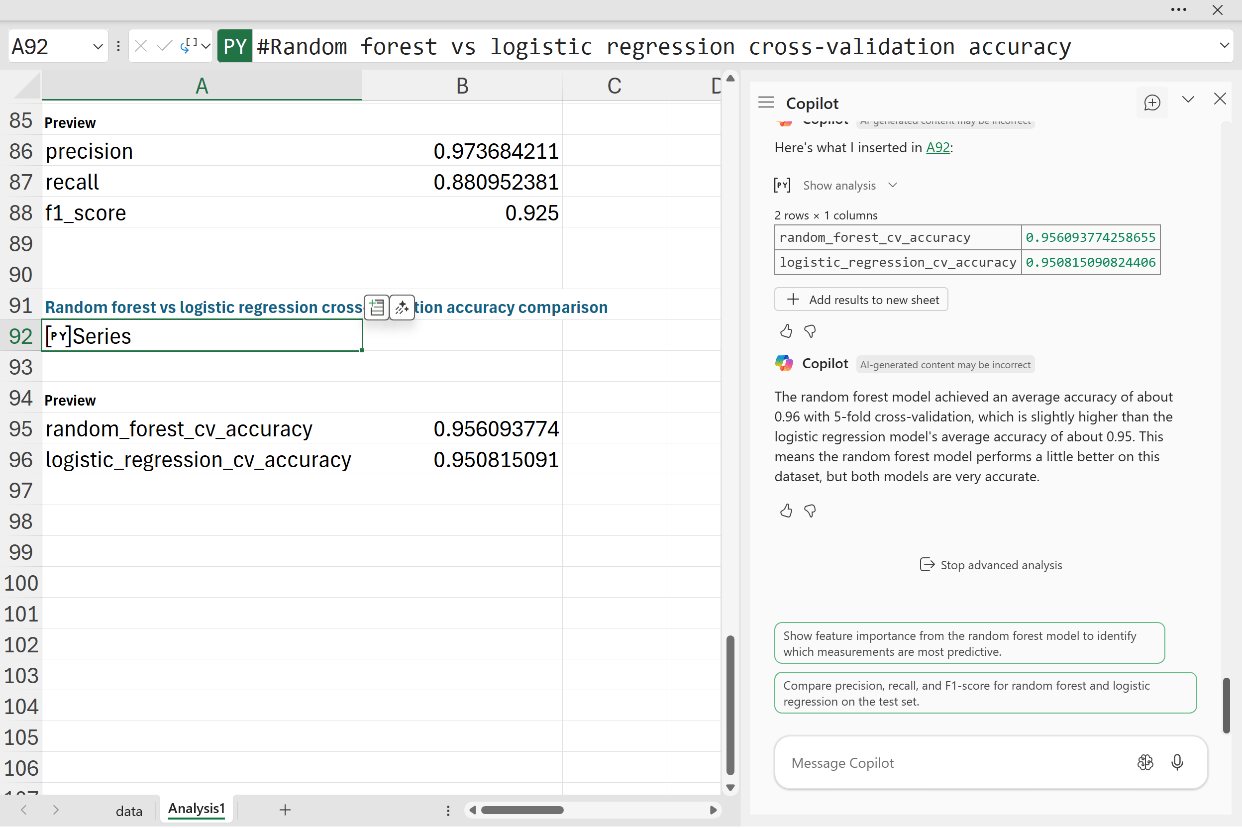
The random forest model reached an average accuracy of about 0.96, compared to about 0.95 for logistic regression. The difference is small, but it shows that the random forest has a slight edge on this dataset. Both models, however, are performing at a very high level.
This comparison is useful because it shows how even a simple baseline model like logistic regression can hold its own against more advanced approaches. For a dataset like this, where the signal is fairly strong, logistic regression is already good enough. The random forest squeezes out a little more accuracy, but both models give us confidence in predicting whether a tumor is benign or malignant.
Conclusion
With these examples, you’ve seen how Copilot and Python in Excel can significantly extend your analytical capabilities without leaving Excel. While Excel’s built-in modeling tools are powerful, they fall short when it comes to the deeper validation metrics. But by adding Python into your workflow, these previously complex methods become straightforward and accessible.
Keep in mind that this walkthrough was just the beginning. For instance, we didn’t explore the coefficients of our logistic regression model. Understanding which variables carry the most predictive weight can add crucial context to your analysis. Explainability is especially valuable in fields like healthcare, finance, or customer analytics, where decision-makers need clarity behind predictions.
It’s also important to remember that every model comes with assumptions and potential pitfalls. Logistic regression assumes linear relationships and limited multicollinearity among predictors. Random forests, while powerful, might sacrifice some transparency. The dataset itself might contain quirks or biases that affect results, so always dig deeper into data quality.
Ultimately, the ability to conduct this type of rigorous validation and deeper analysis directly inside Excel can transform how confidently you approach your everyday data analysis tasks. With Copilot and Python, Excel users can tackle advanced modeling challenges that used to require specialized software. It’s a fantastic leap forward, opening up exciting possibilities for deeper insights, clearer explanations, and better decisions, all within the familiar Excel environment.