
For years, running a logistic regression in Excel meant relying on add-ins like XLMiner or the Analysis Toolpak. They worked in a basic sense, but they were rigid and opaque, and they didn’t give analysts what they really needed: a clear, interpretable model that supports real decision making.
Python in Excel and Copilot’s Advanced Analysis mode change that entirely. Instead of struggling with the tool, we can focus on the actual analytical work. We can explore patterns, test ideas, understand why outcomes occur, and build models that are transparent and easy to explain.
To see this in action, we are using a simple but realistic dataset from a social network advertising scenario. Each row represents a user who was shown an ad, along with information such as gender, age, and estimated salary, and a binary indicator showing whether they purchased the product. The structure makes it ideal for a first logistic regression example.
You can download the exercise file below to follow along in Excel, run the model with Python, and explore the results with Copilot.
If you haven’t set up a dataset to use with Advanced Analysis in Copilot yet, this post will walk you through exactly how to get started:
Before we start prompting, it helps to get clear on what logistic regression actually does. Logistic regression predicts the probability of a binary outcome. These are situations with two possible results such as yes or no, purchased or not purchased, or clicked or not clicked. Linear regression estimates continuous values like income or price, while logistic regression tells you how likely an event is to occur.
In this dataset, each row represents a user who saw a social network ad. We know basic attributes like age, gender, and estimated salary, along with a simple outcome that indicates whether they purchased the advertised product. Logistic regression helps us understand how those characteristics influence the chance that someone converts. Instead of guessing that, for example, higher income users might be more willing to buy, the model quantifies how much each factor matters.
Exploring the data for logistic regression
First things first: your data needs attention before modeling. Logistic regression comes with certain assumptions about the data, and it’s crucial to meet them for meaningful results. Let’s prompt Copilot to guide us through the necessary preprocessing steps:
“Check the dataset for missing values, outliers, and imbalanced target classes. Recommend data preprocessing steps needed before running logistic regression.”

Copilot reported no missing values and no outliers, but it did flag a class imbalance in the Purchased column. We have 257 zeros and 143 ones. This is a mild imbalance, not a crisis. Logistic regression can handle a split like this, so you can continue without immediately fixing anything. The imbalance only affects how the model treats its default prediction and how you interpret accuracy, false positives, and false negatives.
If you want to experiment with balancing the classes, Copilot can walk you through it with a simple prompt like “Use Python in Excel to apply oversampling or undersampling to the Purchased column and explain the tradeoffs.” It keeps the focus on understanding the workflow rather than jumping into advanced techniques.
Next, I asked Copilot to take a look at the numeric features more closely. Distributions matter in logistic regression because extreme skew or scale differences can quietly pull the model off course. So I prompted it with:
“Show the distribution of numeric features and recommend any transformations that would help logistic regression perform better.“

Copilot returned histograms for Age and EstimatedSalary. Age looks fairly even across the range, but EstimatedSalary tilts to the right with a long tail. Copilot suggested scaling both features and possibly applying a log transform to EstimatedSalary if that skew becomes an issue. This is a helpful reminder that logistic regression works best when numeric predictors are on comparable scales and do not contain large distortions. By checking these distributions early, you avoid surprises later when interpreting coefficients or diagnosing model performance.
Building the logistic regression
With the distributions checked, we have a few mild issues to be aware of, but nothing that stops us from moving forward. Age looks fine, EstimatedSalary is a bit skewed, and the class balance leans toward zeros, but none of these are severe enough to pause the workflow. This is exactly the kind of dataset where you can keep going and let the model show you whether any of these concerns actually matter.
Rather than hand-picking variables or writing your own encoding steps, it is easier to let Copilot build the first version of the model. I asked it to fit a baseline logistic regression and walk through which predictors matter:
“Fit a logistic regression model predicting customer purchase using the other available features. Explain the importance of each predictorc and identify which predictors are statistically significant.”

Copilot returned a clean summary table showing the coefficients, standard errors, z-scores, p-values, and confidence intervals. From this first pass, Age and EstimatedSalary clearly stand out with very small p-values, which means they contribute meaningfully to the likelihood of purchase in this dataset. Gender, on the other hand, has a much higher p-value and does not appear to be statistically significant. That is perfectly normal. Baseline models like this often reveal which features actually matter and which ones quietly fall away once the math weighs them properly.
Diagnosing and interpreting model performance
Once the model is built, the next step is to understand how well it actually performs. Copilot can take care of the heavy lifting, so I asked it to explain the results in plain language:
“Visualize the confusion matrix for this logistic regression model and explain, in plain language, what each metric (accuracy, precision, recall, F1, false positives, false negatives) reveals about the model’s predictive strength and weaknesses.”

Copilot returned a confusion matrix along with a clear explanation of each metric. This model gets about eighty five percent of predictions right, which tells us it is generally reliable for this dataset. Precision shows that when the model predicts a buyer, it is correct most of the time. Recall shows how many actual buyers the model manages to catch.
The F1 score summarizes both perspectives and gives a sense of overall balance. The false positives and false negatives are especially useful because they show exactly how the model is getting things wrong. In this case the model tends to miss some actual buyers, and it occasionally predicts purchases that never happen, but overall the pattern is solid for a simple first pass.
This is the point in the workflow where you start making decisions about whether the model is good enough or whether you need to refine it further with scaling, transformations, threshold adjustments, or feature engineering.
Checking the model’s assumptions
Up to this point, we have focused on the data itself. At the beginning of this walkthrough, we checked for missing values, outliers, skewed predictors, and class imbalance. Those steps help us understand the raw material before building anything. Now that we have a fitted model, the focus shifts. We are no longer asking “Is the data clean enough to start modeling?”
We are now asking a different question: “Does the model we built actually satisfy the assumptions that logistic regression relies on?” To dig into this, I asked Copilot to evaluate the assumptions directly:
“Explain the assumptions underlying logistic regression. Check these assumptions using our dataset and discuss any potential issues identified.”

Copilot checked the correlation matrix, confirmed that multicollinearity was not a problem, and then ran the Box-Tidwell test to assess the linearity of each predictor with the logit. This is an important distinction from earlier. Before, we looked at histograms simply to understand the shape of the variables. Here, the test is far more targeted. It examines whether the relationship between each predictor and the log odds of purchase behaves in the way logistic regression expects.
In this case, the linearity assumption appears to be violated for EstimatedSalary. The interaction term is statistically significant, which suggests the logit may curve rather than follow a straight pattern. That does not break the model, but it does tell us that the EstimatedSalary relationship might not be fully captured without a transformation or a nonlinear term. Age, on the other hand, looks fine, and the lack of strong correlations means multicollinearity is not a concern.
These checks help us understand not just what the model predicts, but how trustworthy those predictions are. From here, we can decide whether to refine the model, transform variables, or move on to interpreting and communicating the results
Business interpretation and application
At this stage, we have explored the data, fit the model, checked performance, and verified the key assumptions. The final step is the one that actually matters to stakeholders. A model is only useful if someone can act on it. Copilot helps bridge that gap by turning statistical output into business guidance. I asked it to interpret the model in practical terms:
“Provide a clear, actionable interpretation of the most influential features from the logistic regression. Explain what these results mean for business decisions related to customer retention and marketing strategy.”
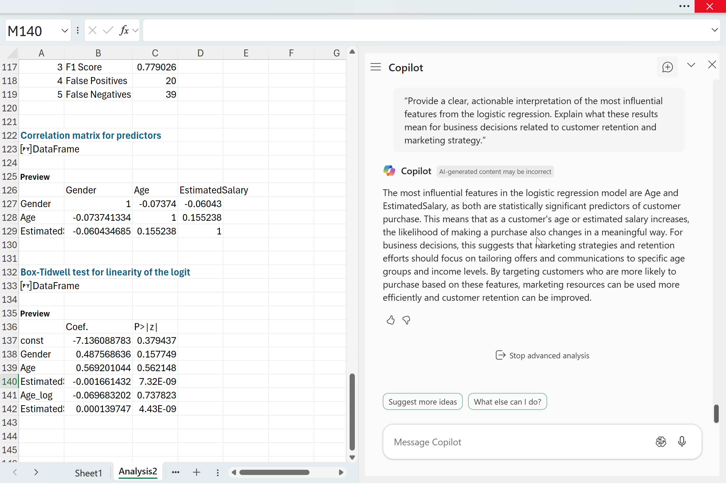
Copilot highlighted Age and EstimatedSalary as the two most influential predictors. Both are statistically significant, which means they have a dependable relationship with purchase likelihood. As either variable increases, the probability of purchase shifts in a meaningful way. For a business audience, this translates into simple guidance. Customer behavior varies across age ranges and income levels, so marketing efforts are more effective when they are tailored to those segments. High-income customers may respond differently to promotions than lower-income customers, and certain age groups may be more receptive to specific products or messaging.
By identifying which groups are more likely to convert, a company can allocate its marketing budget more efficiently and strengthen retention among high-value customers. This is where logistic regression becomes more than a math exercise. It becomes a decision tool. And with Copilot handling the technical translation, analysts can focus on crafting recommendations that are actually useful to the business.
Model refinement and improvement
Once you have a basic interpretation of the model, the natural next question is whether it can be improved. Copilot can help you explore those possibilities just as easily as it handled the diagnostics and interpretation. I asked it:
“Suggest ways to improve model performance further. Should we add interaction terms, polynomial features, or apply feature selection techniques? Guide me through these options.”
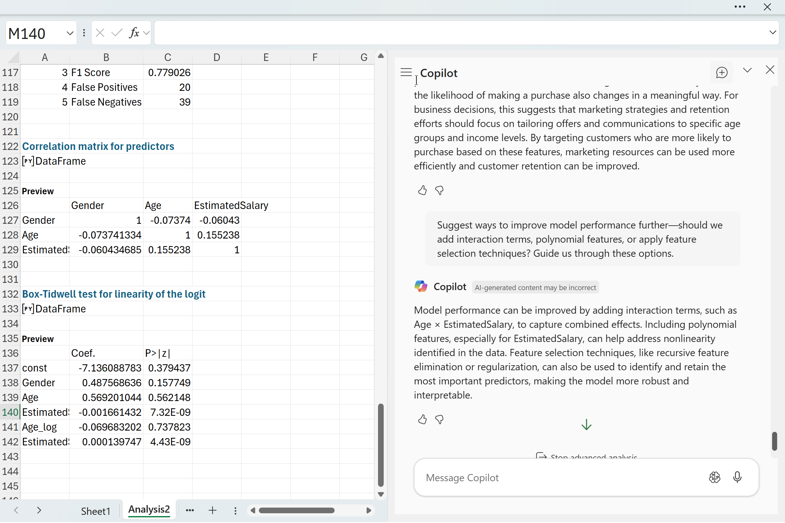
Copilot suggested several paths forward. Interaction terms like Age × EstimatedSalary can capture effects that a simple additive model might miss. Polynomial features can help address the nonlinear behavior we saw with EstimatedSalary in the Box Tidwell test. Feature selection methods can refine the model by focusing on the strongest predictors while reducing noise. These are the kinds of steps analysts consider once the baseline model is understood and the assumptions have been checked. None of them guarantee better performance, but they offer structured ways to experiment and push the model further.
Conclusion
Logistic regression becomes much more approachable when Python and Copilot are available directly inside Excel. You can explore patterns, check assumptions, and interpret results without switching tools or fighting with add-ins. Copilot handles the mechanics and keeps the explanations clear, so you can focus on what the model is actually telling you.
At the same time, this workflow shows that even a clean dataset has limits. Logistic regression depends on certain assumptions, and real data does not always line up perfectly. EstimatedSalary’s nonlinear behavior is a good example. The model still works, but it hints at opportunities to improve things through transformations, interactions, or more flexible approaches. Copilot helps you explore those options, but your judgment guides the final call.
The big takeaway is that building and understanding models in Excel is no longer a chore. With Python and Copilot, you can create an interpretable model, evaluate it, and translate the results into real business insight. From here, you can refine the model, test new features, try different thresholds, or compare logistic regression with tree-based methods. Whatever direction you take, this workflow gives you a solid foundation to keep going.