Pivoting on Text in Excel: Awards by Player PivotTable

This post is inspired by a Mr. Excel tutorial on using “text instead of numbers in a Pivot Table.”

Our goal is to create a Pivot-Table like report that creates a comma-separated list of players who won any given award in a given year. We will filter and merge information from these two tables using Get & Transform, then use Excel’s Data Model to pivot on text. This is an added functionality over base PivotTables which do not allow you to pivot on text in this manner.

Follow along with the completed workbook here.

1. Download Lahman baseball data

Once again we use the 2017 .csv version of the Lahman baseball dataset, this time the People.csv and AwardsPlayers.csv. Open a new workbook and paste each dataset into its own worksheet. Convert the datasets into Excel Tables with the Ctrl + T keyboard shortcut.

2. Filter the Awards dataset

The AwardsPlayers dataset records awards won by players going back to the 1870s. We will focus only on awards won since 2010.

Go to Data | From Table to bring up Power Query where you can then click on the yearID filter and filter out years before 2010.

When you are finished, select Close & Load To, then select “Only Create Connection.”

3. Merge the Players dataset

Currently the AwardsPlayers dataset does not include the player’s given names, only their PlayerIDs (used as a primary identifier in the Lahman datasets).

To get players’ given names we will bring the Players dataset to Power Query similarly by selecting Data | From Table. Then again select Close & Load and Only Create Connection.

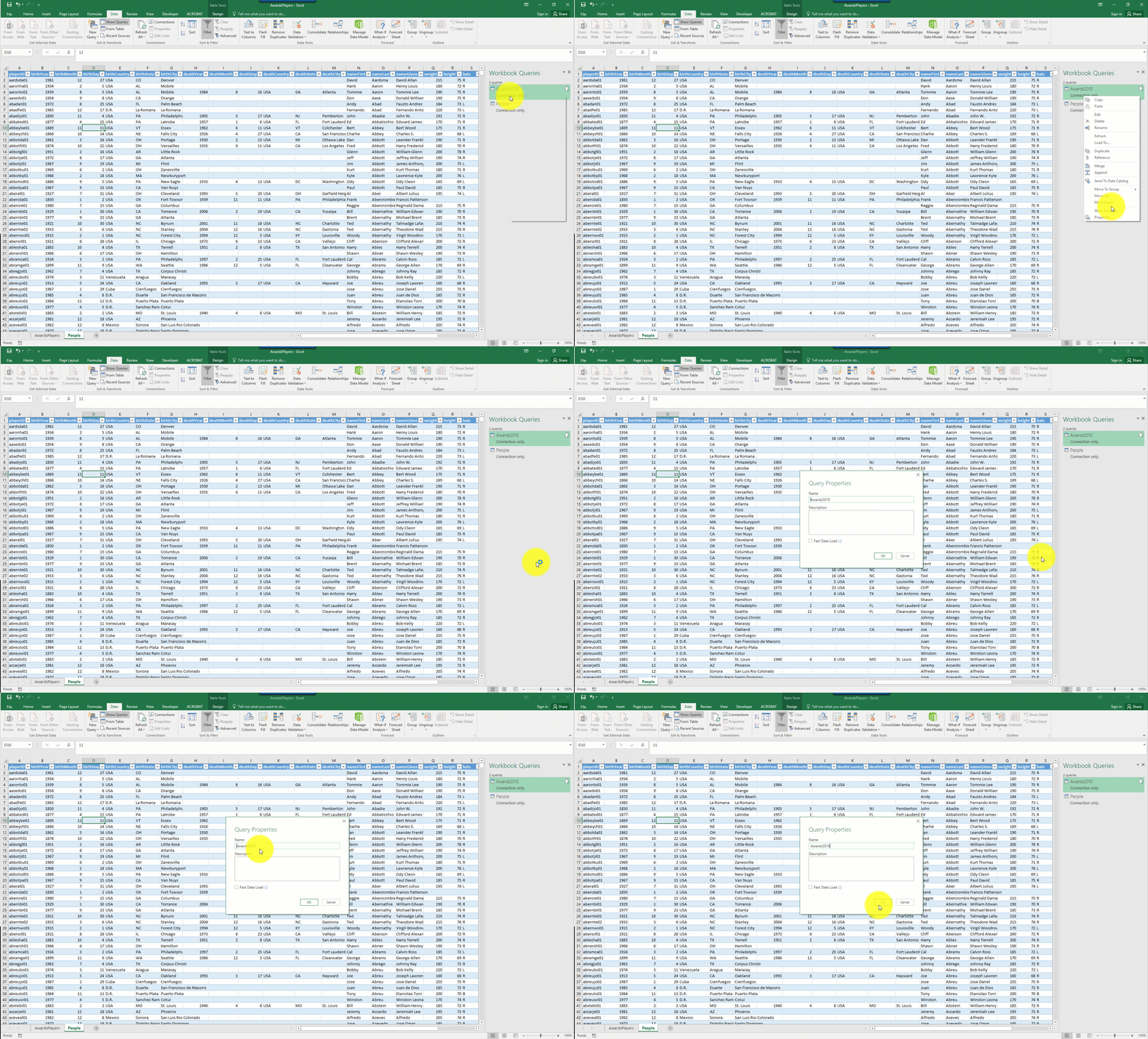
You should now see two tables listed on the right-hand side of your workbook entitled “Workbook Queries.” You can change the names of your queries by right-clicking on the query and heading to “Properties.”

Change them to something related to your datasets, such as “Awards2010” and “Players.”

Now we are finally ready to merge. Go back up to Data | New Query, then select Combine Queries | Merge.

Here we will get a pop-up box asking us which queries we want to merge. Selecting your awards then your players datasets, Excel will assume you want to perform a Left Outer join. This is what we want because we want to keep all Award records and get as much Player information as we can.

Next we tell Excel what field to merge by. We will use the playerID field which is an identifier across tables. Click on the field in each table.

You will get a table with 502 records (as of 2017).

Click on the filter of the “People” column which has been appended to your Awards dataset to select which fields will be included in your table.

Close and load the query to an Excel table. This table then becomes the basis for our “Pivot by Text” report.

4. Create a Full Name Column

The last column of your new query is named “People” and contains all of the information from the People dataset for each playerID. We want a “First Name Last Name”-type field, so we will select the “nameFirst” and “nameLast” fields from the People dataset.

We will then head over to Add Column | Custom Column on the home ribbon and create a new column, “FullName.”

I include a screenshot below of the Custom Column syntax. Similar to stringing text together in Excel, I use the & character and a space in quotation marks to create this field.

Close and load this table to our workbook.

5. Set up Data Model

We finally have our raw data of player names and awards. Now we want to summarize this data into a PivotTable listing the names of players who won a given award in a year.

Setting up the PivotTable, make sure to check “Add this data to the Data Model.”

5. Add Calculated Field

Now we will add a calculated field to the Data Model. Right-clicking on our “Merge1” query in the PivotTable fields, select “Add Measure.” We will now use the DAX language to add a measure that will allow us to concatenate together a list of names separated by a comma and a space.

I have included a screenshot of the DAX formula below because there is a lot going on here. Essentially we are creating a measure allowing us to concatenate items in the nameGiven field with a comma and a space.

6. Pivot to your heart’s content.

It took some hand-wringing but now we have a list of full names of players who won a given award in a given year that we can report in a Pivot Table. Notice that we even get “subtotaled” aggregated lists of names too!

Thanks again to Mr. Excel for the inspiration for this post combining baseball data, Get & Transform and the Data Model.