Power Pivot is a fantastic tool that lets you build relational models right from Excel. This negates the “death by VLOOKUP()” that many large workbooks face — defining relationships across multiple tables is just more efficient than creating one giant “Frankentable.”
That being said, sometimes having one field “looked up” into another table can be necessary, whether for aesthetic or calculation reasons. Fortunately, the RELATED() function exists to, as the documentation puts it, “return a related value from another table.”
Let’s see how it works using a simple student gradebook example.
Establishing the relationship
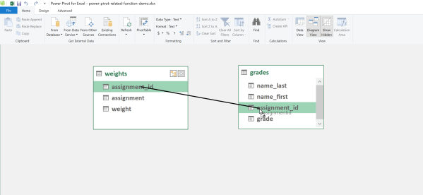
The RELATED() function only works with an established relationship between tables. Think of the column(s) that establish these relationships as like your lookups — they are the ones found across tables. In this case, assignment_id is found in both weights and grades, so we’ll head over to Diagram View in Power Pivot and establish the relationship:

Using RELATED() in a calculated column
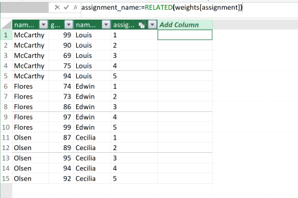
With the relationship established, we’re now free to use the RELATED() function in our calculations and measures. Start by going over to Data View in the Power Pivot editor. We would like to “look up” the assignment column from weights into the grades table so that it’s easier to know which assignment_id corresponds to which assignment.
RELATED() only takes one argument: what column from the related table to you want to look up? In this case, it’s assignment so our formula will look like this:
assignment_name:=RELATED(weights[assignment])
Go ahead and hit Enter to fill the formula down and create this calculated column. The assignment name has now been looked up into this table.
Using RELATED() in a calculated measure
It’s also possible to use the RELATED() function inside a calculated measure. Remember, creating a calculated column means that data persists regardless of what you do with the model. Calculated measures are more efficient as they are only derived on-demand. Just like too many VLOOKUP()s can bloat a workbook, the same can be said for too many calculated RELATED() columns.
From inside the Power Pivot editor, go ahead and click PivotTable to insert a Power PivotTable into your workbook. We will now create a calculated measure by going back to the home ribbon and Power Pivot > Measures > New Measure.
We will use the RELATED() function to “look up” the respective weight for each assignment type and create a weighted grade average using the iterator function SUMX():
=SUMX(grades, [grade] * RELATED(weights[weight]))
We can now set up a PivotTable to view the total semester grade for each student:

If your Grand Total is turned on for this measure, you’ll see the PivotTable takes a sum of the weighted grades rather than averaging them. This can be modified with a bit of DAX wizardry as provided by Rory on the Mr Excel message forums.
Looking up to RELATED()
Whether for a calculated column or measure, RELATED() brings you all the convenience of functionality of VLOOKUP() in the enhanced data model environment. When have you used this function before, or do you have a case where it might be helpful? Let me know in the comments.
