If, as I write in Advancing into Analytics, lookup functions like VLOOKUP() are the duct tape of Excel, then relational joins in Power Query are like a full-on blowtorch, allowing you to contort data sources in an endless variety of ways.
In this post, we’re going to look at a less common but nevertheless powerful join type called the Cartesian or cross join. This join type can be used to find the combination of all items across tables:
Let’s give it a try on this data in Excel Power Query:
Understanding the data
This example is based on an actual client project where I wanted to document all the different combinations of tasks that might need to be performed on a system. What I did was list out each component and the different tasks for that component; here’s a simplified, fictional example that you’ll find in the exercise file:

Rather than list out all the combinations manually, we’ll use cross joins in Power Query to do it for us.
Setting up the crossjoin query
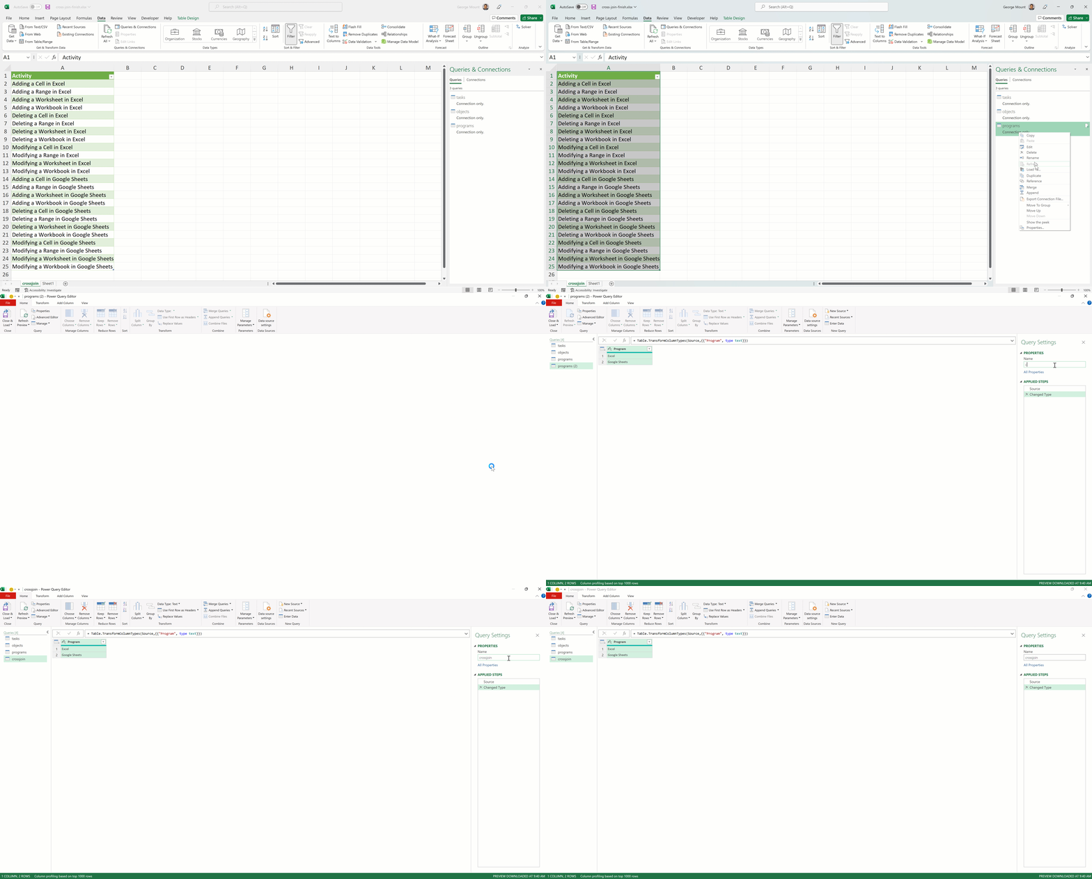
To kickstart this process, go to Data on the home ribbon then Queries & Connections. Right-click on the programs query that has already been set up in the workbook, then select Duplicate.
This will launch the Power Query editor. You can rename the new query crossjoin:

Adding the first cross join
Next, we will cross-join the tasks table to our duplicated program table. If you’ve done an inner or left outer join, for example, in Power Query, you’ll notice the steps here are quite different.
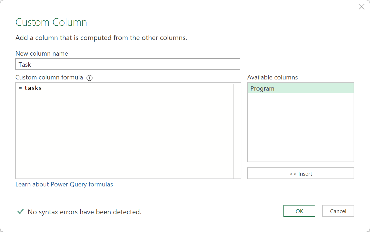
To make the cross join, go to Add Column on the ribbon, then Custom Column. In the Custom column formula editor, simply type tasks (the name of the table we’re joining to). Also, name the custom column Task.

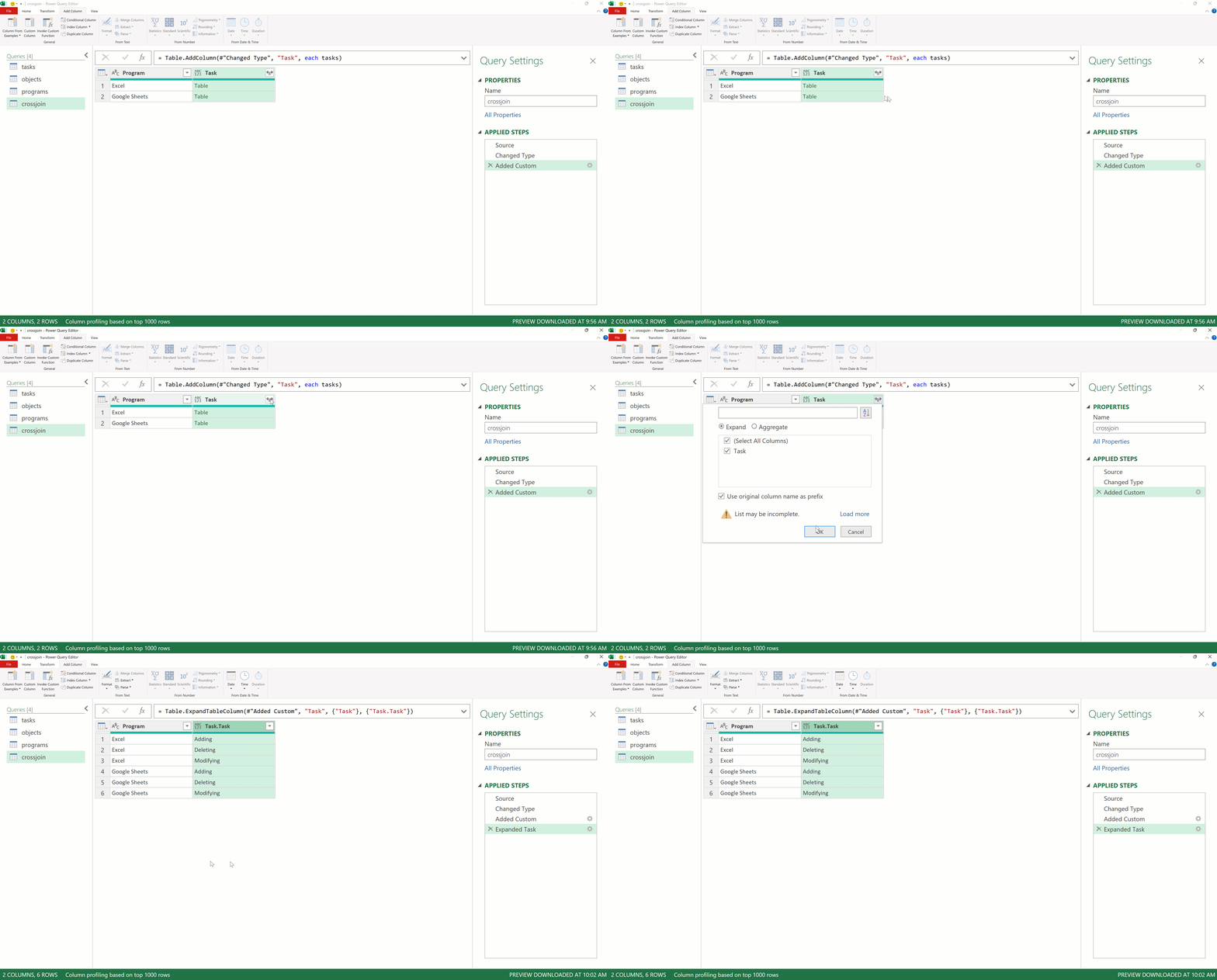
Click OK and it looks like you’ve got a mess on your hands, right? The resulting column simply says Custom with green entries called Table running throughout.
The data you want is actually hiding under this mess… to see it, click the according-looking filter button next to Task and click OK:

Brilliant! You now have a list of the combinations of all Programs and Tasks in the workbook. Go ahead and add the Object column to the table using the same steps and you should see something like this:

Consolidating into one column
Nice! We’ve listed out all the combinations between these three tables. But what I really want is a nice, combined column summarizing the three in proper English, e.g. Adding a cell in Excel, Adding a worksheet in Google Sheets, etc.
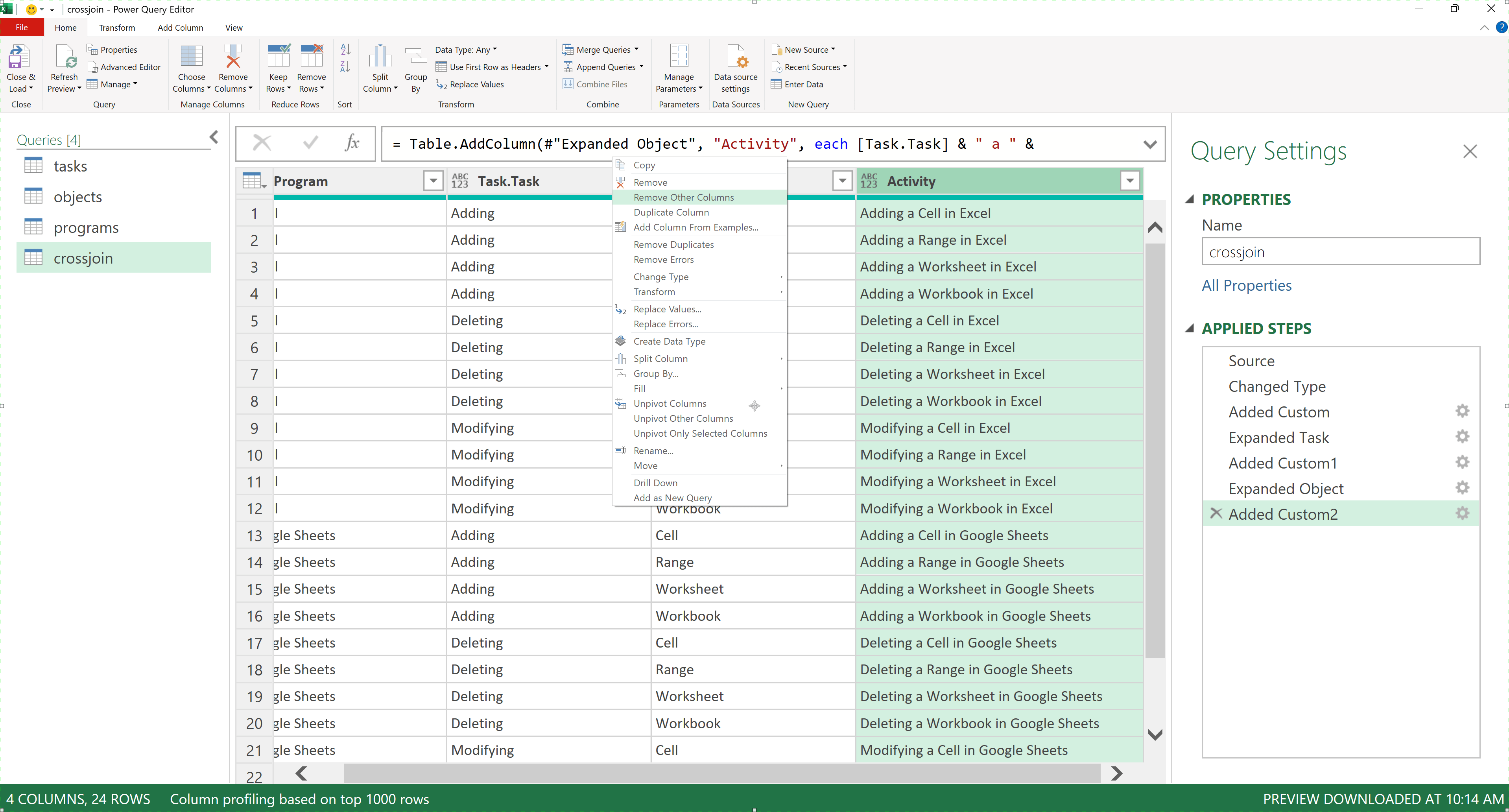
To do this, we can add yet another custom column to the query. Call this one Activity:

Now, we got a little lucky here because each of our objects start with a consonant, so we didn’t have to conditionally control for a versus an in the column. However, this could be taken care of with a conditional column in Power Query.
Because we have our results tidily displayed in one column, we can go ahead and delete the former “helper” columns by right-clicking on Activity and selecting “Remove Other Columns:”

Finally, you can view the results of your handiwork in Excel by going to Home > Close & Load in the Power Query editor ribbon. You should see this result:

From here, we would possibly move the list over to a Word doc or wherever else to begin the documentation. Sure beats writing out all the combinations by hand, right?
You can compare your results to the solution workbook:
Have you needed to perform this type of task before? How did you do it? Are there other more unusual joins in Power Query you’d like to learn more about? Let me know in the comments.
Looking to learn more Power Query? Check out my book Modern Data Analytics in Excel:

