Excel is essential for finance professionals, who are among its most intensive users. Many recent Excel features, like dynamic arrays, are genuinely transforming how they work. Previously, financial models were fragile, static creations that required extensive manual adjustments. Even extending a forecast from something like 5 to 7 years involved tedious rework and hardcoded cells. Dynamic arrays simplify this dramatically.
Here’s an example inspired by materials from Alpha Development, where I serve as a trainer. If you’re in L&D for financial services, I highly recommend connecting with them.
You can download the exercise file below to follow along:
In this example, let’s assume a straightforward commission model. We’ll say there’s a $10,000 contract, and you’ll earn a 3% annual commission on that amount each year. We’re keeping the assumptions simple so we can focus more on how dynamic arrays work rather than the complexity of the financial model itself.
The first step is setting up a sequence from 1 to N, where N is the number of years specified in cell C1. You can easily do this using Excel’s SEQUENCE() function:

Now let’s calculate the face value commissions. The goal here is making this calculation dynamic so it automatically works regardless of how many years the contract runs. A clever trick is to reference a spilled range, specifically cell B7, and multiply it by zero. This generates a dynamic array. Then multiply the initial value by the annual commission rate, giving you that $300 commission each year. Pretty slick!

If you’ve never seen the spill operator used in Excel before, check out this earlier post:
Now let’s calculate the discount rate for each year’s commission, because $300 today isn’t the same as $300 five years from now. But how much less is it really worth? We can dynamically calculate this using the interest rate. This formula leverages Excel’s spill operator (#) to apply a discount factor across all years at once, converting future commissions into their present values. Each year’s commission is then adjusted to reflect its true worth in today’s terms.

Awesome! Now, to finish things off, just multiply these spill ranges together to get your discounted commission payment.

Alright, let’s wrap this up! To summarize, let’s use the spill operator one more time to easily sum up the discounted commissions.

We can also visualize how the present value of that commission changes year over year. And again, this needs to be dynamic. We’ll use a neat trick in Excel to automatically expand the calculation as the number of years changes. (If you thought your financial modeling was already transformed, wait until you see this!)
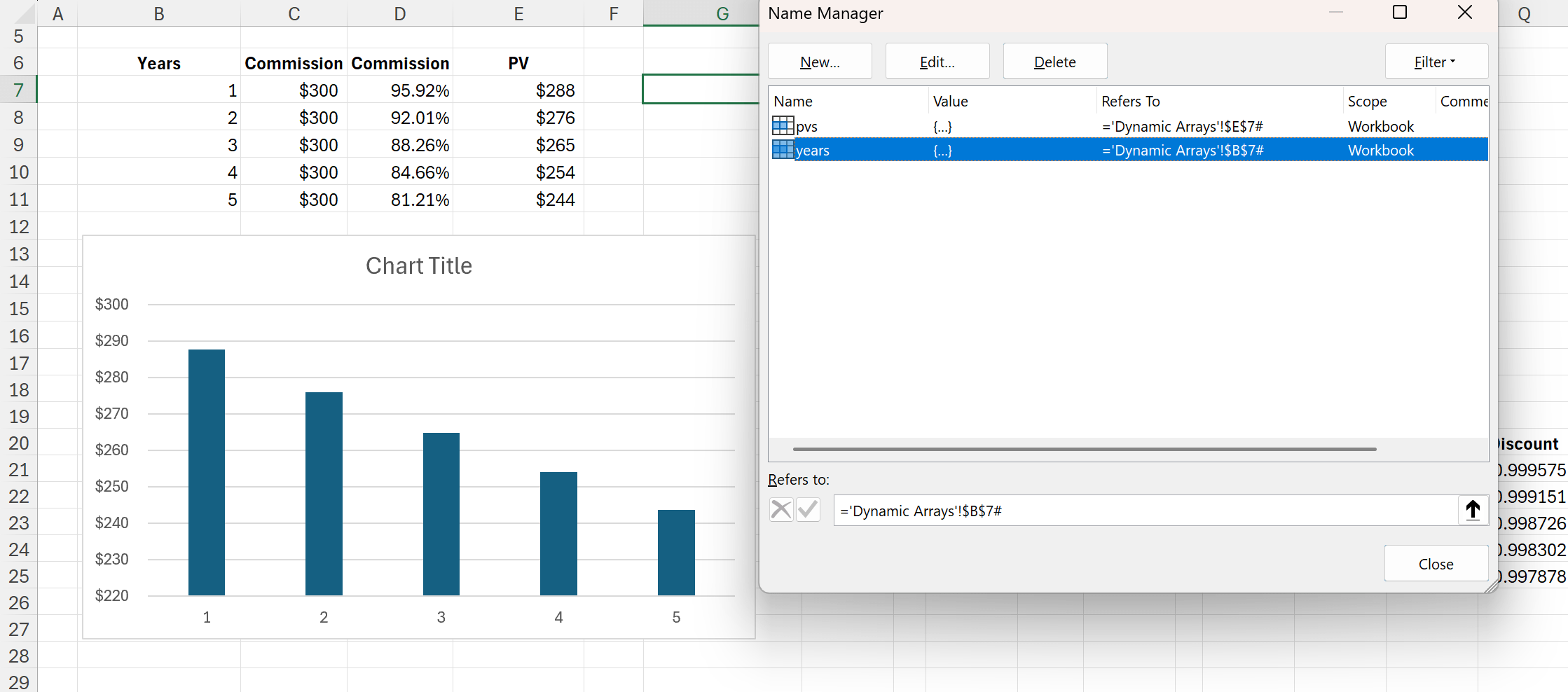
The first step is to name both the PVs and years ranges, making sure to reference the spill range with the spill operator (#). Here’s how it looks in the Name Manager:
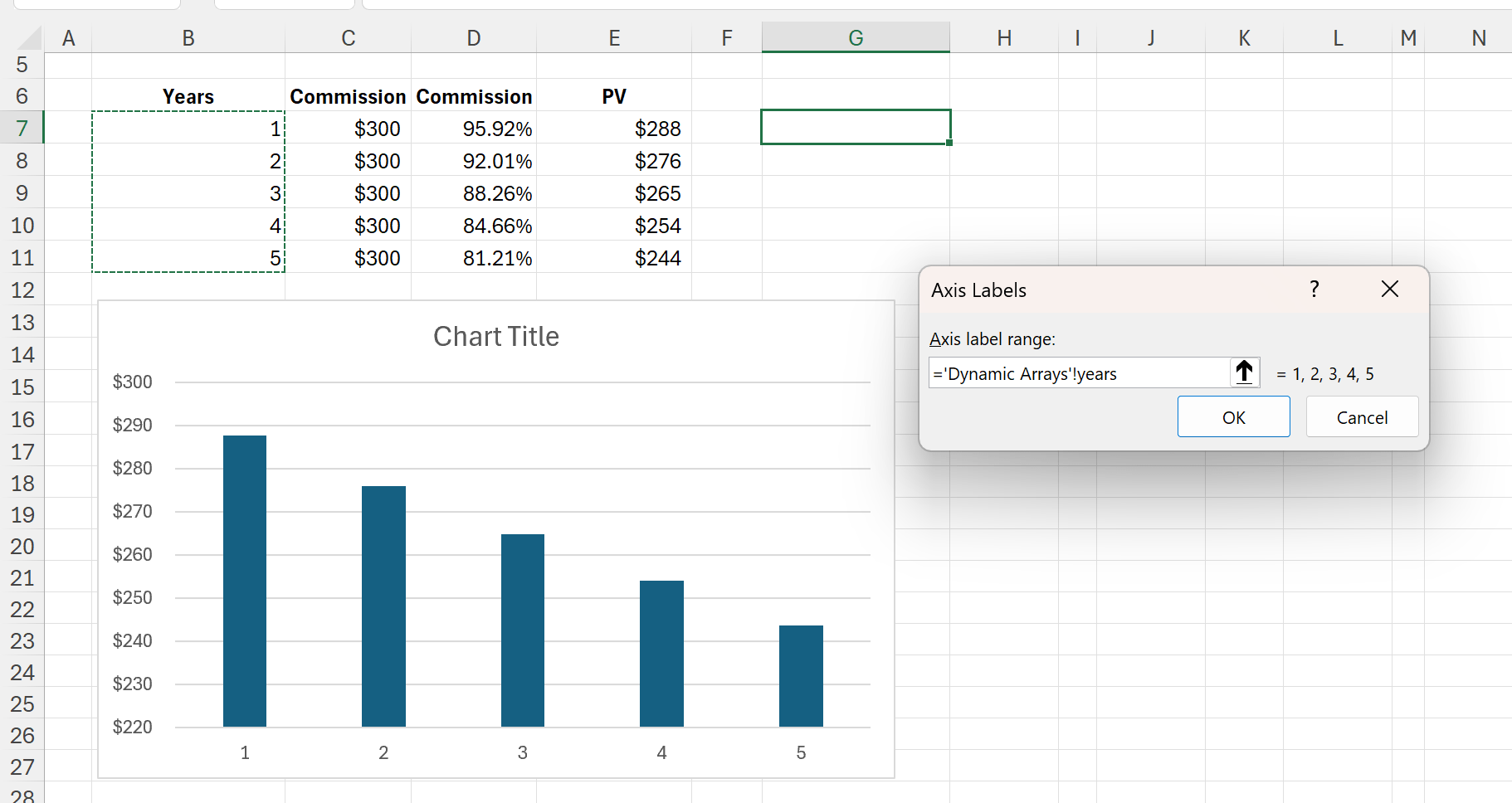
Now, right-click your chart and select Select Data. Instead of pointing to a fixed range, refer to the named ranges you just created. Be sure to include the worksheet name in the reference. Set years as your label range and pvs as your legend entries:
Awesome! Now this setup is fully dynamic. You can adjust the number of years or any of the other parameters and watch everything update instantly:
This model was intentionally simple, but the same principles apply to all sorts of financial models, from cost of capital calculations to income statements and beyond.
Do you have any questions about using dynamic arrays for financial modeling, or dynamic arrays in general? Drop them in the comments!